Complexity & P

Complexity & Computational Model

We have seen that, thanks to the Church-Turing thesis, all computational models as powerful as Turing machines are equivalent in terms of what problems are decidable and undecidable.

However, the efficiency of these solutions can vary on different computational models.

How can we decide $A = \{0^k1^k\; |\; k \ge 0\}$ with a multi-tape Turing machine in linear time $TIME(n)$?

The complexity of a problem depends on the computational model being used.

Complexity of Multi-Tape Turing Machines

We can convert any multi-tape Turing machine into an equivalent single-tape one using the technique discussed when we covered Turing machine variants. The technique is repeated here:

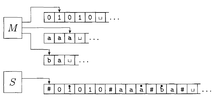
Given some multi-tape Turing machine $M$, we can build an equivalent single tape machine $S$ is defined as follows:

$S =$ "On input $w = w_1w_2...w_n:$

Put the tape into the format described above:

$\#\dot{w_1}w_2...w_n\#\dot{\sqcup}\#\dot{\sqcup}\#\dot{\sqcup}\#\dot{\sqcup}...$
To simulate a single move, $S$ scans the entire tape to see which symbols are under the tape heads (the dotted symbols). It then makes a second pass according to the transition function of $M$ to change the tape: writing new symbols under the tape heads, and moving the dots left or right.
If at any point $S$ moves a tape head to the right onto a $\#$ symbol, it means $M$ has moved the tape head to the end of a tape. So $S$ writes a blank symbol over the $\#$ symbol, shifts the entire rest of the tape one position to the right, and restores the $\#$ symbol. It then continues on where it left off."

How much computational complexity is introduced with this simulation? If the multi-tape Turing machine $M$ runs in $t(n)$ time, how much time is required for the single-tape machine $S$ provided by this construction?

Because $S$ must scan across the tape for each step of the computation, the time required is equal to the time required to scan the tape times the number of steps $t(n)$.

It may seem it takes $\mathcal O(n)$ time to scan the tape, but the operation of $M$ may be increasing the length of the tape as it runs. The maximum amount $M$ can increase the tape is $k \times t(n)$ where $k$ is the number of tapes.

Thus, the time to scan the tape is at most $\mathcal O(t(n))$, and the full running time of $S$ is $\mathcal O(t^2 (n))$.

Complexity of Non-Deterministic Turing Machines

Next, we'll consider a non-deterministic Turing machine. We define the running time $t(n)$ of a non-deterministic Turing machine as the maximum number of steps in any branch of the computation:

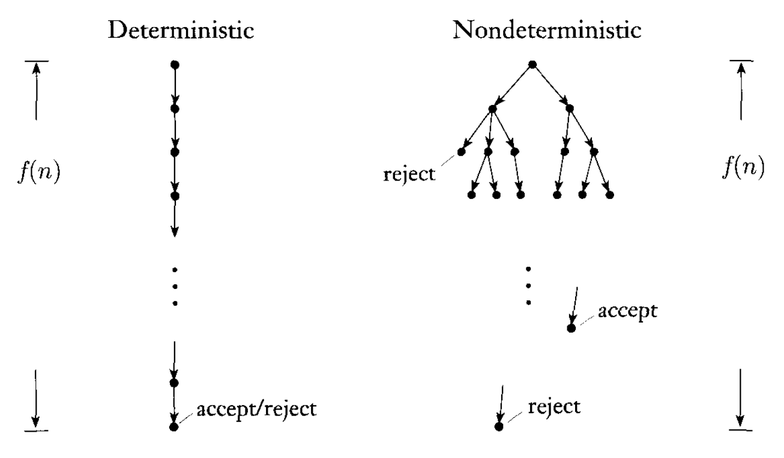
Recall that the algorithm for simulating a non-deterministic Turing machine $N$ on a deterministic Turing machine $D$. It uses a breadth first search of the tree of computation.

If we use this method to simulate $N$ which runs in time $t(n)$, how much time will the deterministic Turing machine $D$ take?

By the definition of a non-deterministic Turing machine complexity, every branch of the tree has length at most $t(n)$. Every node in the tree has at most $b$ children where $b$ is the maximum number of choices at any point in the $N$.

Thus, the total number of leaves in the tree is at most $b^{t(n)}$. The number of nodes in the tree is less than twice the number of leaves. So we can bound it by $\mathcal O(b^{t(n)})$.

The time it takes to travel from the root to any one node is $\mathcal O(t(n))$. Thus the total running time of $D$ is $O(t(n) b^{t(n)})$. This is equal to $2^{\mathcal O(t(n))}$.

The simulation actually uses a three-tape Turing machine. As discussed above, this at most squares the running time, so we have $(2^{\mathcal O(t(n))})^2 = 2^{\mathcal O(2t(n))} = 2^{\mathcal O(t(n))}$.

Polynomial Time

The difference between a single-tape and multi-tape Turing machine is much smaller than the difference between a deterministic and non-deterministic one. We will call polynomial differences in time small, and exponential differences large.

An algorithm that completes in polynomial time is usually useful, whereas an exponential one rarely is.

All reasonable deterministic models of computation are polynomially equivalent. That means that one can simulate the other using only a polynomial increase in running time.

The Class P

$P$ is the class of languages that are decidable on a deterministic single-tape Turing machine in polynomial time:

$P = \bigcup\limits_{k} TIME(n^k)$

That is, $P = \{n, n^2, n^3, n^4...\}$.

$P$ is a useful class to talk about because:

$P$ is invariant to the model of computation we discuss.
$P$ mostly corresponds to the set of problems that have "feasible" solutions.

The Path Problem

One example of problem in $P$ is the $PATH$ problem:

$PATH = \{\langle G, s, t\rangle\; |\; G$ is a directed graph that has a path from $s$ to $t\}$.

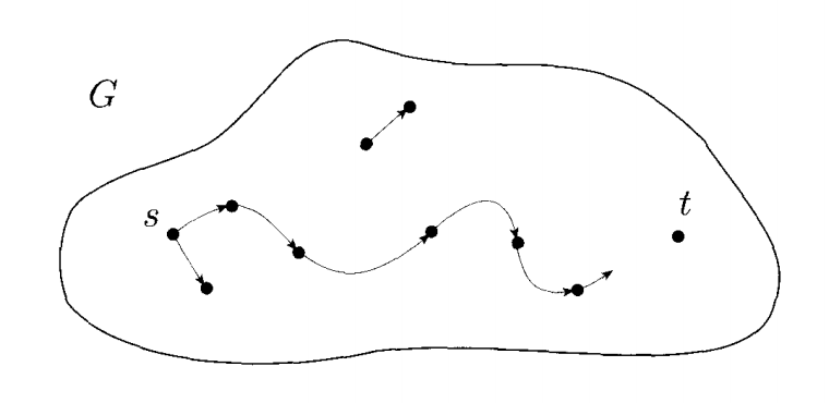
How can we show that $PATH$ is in $P$?

The following algorithm decides $PATH$:

$M =$ "On input $\langle G, s, t \rangle$:

Place a mark on node $s$.
Repeat until no nodes are marked:
1. Scan all edges of $G$. If an edge $(a, b)$ is found where $a$ is marked, and $b$ is unmarked, mark node $b$.
If $t$ is marked, accept. Otherwise reject.

What is the complexity of $M$?