Turing Machine Variants

Overview

There are many alternatives to Turing machines. Today we will discuss some along with the languages they recognize.

It turns out that the simple Turing machine definition we looked at is extremely robust. The extended models do not offer any increased ability to describe languages.

"Stay Put" Turing Machines

As a simple example, consider a "Stay Put" Turing machine, which is able to keep its tape head in the same location, in addition to being able to move left or right.

Formally, we would say the transition function is:

$\delta : Q \times \Gamma \rightarrow Q \times \Gamma \times \{L, R, S\}$

Where 'S' indicates the tape head should stay where it is.

How can we show that a "Stay Put" Turing machine is equivalent to a regular one?

Multi-Tape Turing Machines

A multi-tape Turing machine is one that has $k$ tapes for reading and writing information, instead of only one.

The first tape is initialized with the input, and the rest are initially empty.

Formally, the transition function is:

$\delta : Q \times \Gamma^k \rightarrow Q \times \Gamma^k \times \{L, R\}^k$

We can transition based on all $k$ current input symbols, write a symbol to each of the $k$ tapes, and move each of the $k$ tapes either left or right.

Despite these added abilities, multi-tape Turing machines are no more capable than regular ones.

To prove this, we will need to show that any multi-tape Turing machine can be simulated with a standard one. This is done in the following manner:

Store the contents of all $k$ tapes on the one tape, separated by the # symbol.
Keep track of the tape heads using "dotted symbols". Each of these is a new input symbol which is identical to a symbol in $\Gamma$, with a dot over it.
Have the machine execute the tape operations of the multi-tape machine one by one.

The following figure shows an example of a computation on a multi-tape Turing machine, and the equivalent computation on a single-tape one.

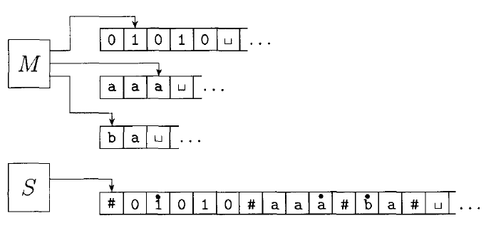
Given some multi-tape Turing machine $M$, we can build an equivalent single tape machine $S$ is defined as follows:

$S =$ "On input $w = w_1w_2...w_n:$

Put the tape into the format described above:

$\#\dot{w_1}w_2...w_n\#\dot{\sqcup}\#\dot{\sqcup}\#\dot{\sqcup}\#\dot{\sqcup}...$
To simulate a single move, $S$ scans the entire tape to see which symbols are under the tape heads (the dotted symbols). It then makes a second pass according to the transition function of $M$ to change the tape: writing new symbols under the tape heads, and moving the dots left or right.
If at any point $S$ moves a tape head to the right onto a $\#$ symbol, it means $M$ has moved the tape head to the end of a tape. So $S$ writes a blank symbol over the $\#$ symbol, shifts the entire rest of the tape one position to the right, and restores the $\#$ symbol. It then continues on where it left off."

Non-deterministic Turing Machines

A non-deterministic Turing machine is one which can take one of several actions at each step in the computation.

The transition function is defined as:

$\delta : Q \times \Gamma \rightarrow \mathcal P(Q \times \Gamma \times \{L, R\})$

Just like an NFA, the computation of a non-deterministic TM is a tree, where each branch is a possible action. If any branch results in an accept, the machine accepts the input.

Non-deterministic Turing machines are no more powerful than deterministic ones.

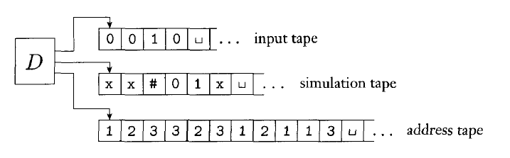
To show this, we will simulate a non-deterministic machine $N$ with a deterministic one, $D$. In order to accomplish this, the deterministic Turing machine will need to search the entire tree of computation looking for an accept state.

$D$ uses three tapes (which could be collapsed into one as described above):

The input tape stores the input string and is not altered.
The simulation tape contains a copy of $N$'s tape on some branch of the computation.
The address tape keeps track of where $D$ is in the tree of $N$'s computation.

At each step in the computation $N$, there will be a set of transitions we could make. We will number these $1 - b$, where $b$ is the largest number of options any state has.

The string stored on the address tape keeps track of the sequence of choices we have made. For example $132$ means that we took the first option initially, then the third option, and finally the second.

$D =$ "On input $w$:

Initially, tape 1 contains the input $w$, and tapes 2 and 3 are empty.
Copy tape 1 to tape 2.
Use tape 2 to simulate $N$ with input $w$ on this branch of its computation. Before each step, consult the next symbol on tape 3 to determine which choice to make among those allowed by the transition function of $N$. If no more symbols are on tape 3, or if the choice given is invalid, abort this branch, and go to step 4. If we get to the reject state, abort and go to step 4. If we get to the accept state, accept.
Replace the string on tape 3 with the next string lexicographically, and go to step 2.

It may take a long time, but $D$ will eventually try every branch of computation in $N$. If $N$ can possibly accept its input, $D$ will as well.

Enumerators

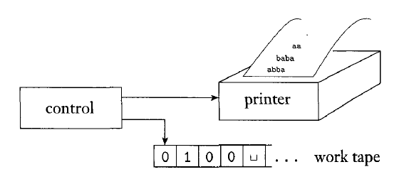
An enumerator is a Turing machine with a printer attached. The enumerator starts with no input on its tape. Rather than accept or reject strings, the enumerator prints out a set of strings which is the language of the enumerator.

The enumerator may elect at any point to print the string on its tape.

Every enumerator has an equivalent Turing machine that recognizes the language it generates. The following Turing machine $M$ recognizes the language produced by some enumerator $E$:

$M =$ "On input $w$:

Run $E$. Every time $E$ outputs a string, compare it with $w$.
If $w$ ever appears in the output, accept.
If $E$ halts before this happens, reject.

Also, every Turing machine has an equivalent enumerator that generates the language it recognizes. The following enumerator $E$ generates the language recognized by some Turing machine $M$:

Say that $s_1, s_2,...$ is a list of all strings in $\Sigma^{\ast}$.

$E =$

Repeat the following for $i = 1, 2, 3...$

Run $M$ for $i$ steps on each input $s_1, s_2, ..., s_i$.
If any computation accepts, print out the string that was accepted.

Here $E$ is careful to avoid infinite looping in $M$ by limiting the number of steps that are executed.

Equivalence with Other Models

Many other general models of computation have been proposed. Some are similar to Turing machines. Others (like the lambda calculus of Alonzo Church) are much different.

All of these models that have unrestricted access to unlimited memory are equivalent.

This means that the set of things that can be computed is independent of the actual computer model being used. Anything that can be computed with a powerful super-computer can be computed with a simple Turing machine.