Huffman Coding

Introduction

Huffman coding is a simple method of data compression. In data compression we want to represent some information in the smallest memory space possible. There are two main types of compression:

Lossy: some data is lost in the process (.jpg, .mp3, etc.)
Lossless: no data is lost in the process (.png, .flac, .zip etc.)

Huffman coding uses lossless compression.

We will use the following terms when discussing encoding:

Symbol
A symbol is a representation of a single piece of information.
Code
A code is the set of possible symbols.
Sentence
A sentence is a sequence of symbols representing some message.

For example, if we have the code:


{3, 7, 14, 18, 29, 35, 42, 56}

Then the following are sentences:


7, 42, 3, 35, 56, 3
42, 7
3, 3, 3, 35

Prefix Codes

A prefix code is a set of words with the prefix property. This states that for each word in the code, no valid word is the prefix for another.


{4, 5, 34, 37, 95}

Is a prefix code because none of the words are the prefix of another. However:


{4, 5, 54, 37, 95}

Is not a prefix code because "5" is the prefix of another word "54".

The benefit of a prefix code, is that, given the code, we can identify the individual words without breaks:


Code: {4, 5, 34, 37, 95}
Sentence: 45349553745

What are the symbols in this sentence?

For compressing data, this means we don't have to include separators in the output.

General Idea

The idea behind Huffman coding is that certain pieces of information in the input are more likely to appear than others. We will give these common symbols shorter codes to conserve space.

For simplicity, we will consider lower-case letters as our words. In English, for example, some letters are much more likely to appear.

This is true for most types of data, allowing for compact representations.

Binary Tree Representation

A Huffman code works by creating a tree to store the possible symbols. The code used for each symbol is the path from the root to that symbol. For the text:


this is a test

We have the symbols:


{t, h, i, s, a, e}

Then we find the frequency of each:


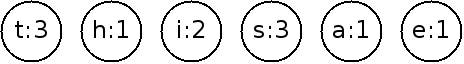
{t:3, h:1, i:2, s:3, a:1, e:1}

Now we will and create nodes for each symbol:

There are 6 nodes, one for each symbol. Each node contains the symbol,
along with the count of each symbol — Nodes of the tree

Building The Tree

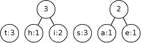
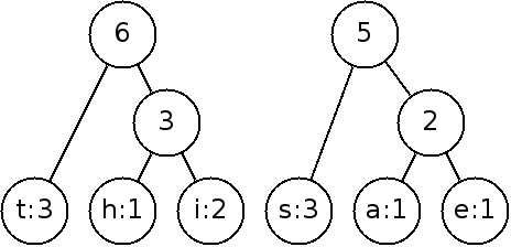
Next, we will construct the tree by repeatedly joining the nodes with the smallest weights until it is a full tree. When there is a tie, it doesn't matter which weights we pick.

Two nodes with the smallest counts are connected as children
of a parent node. That parent's count is the sum of the two childrens
counts — Step 1

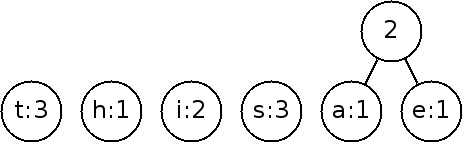
The weight of the new node is that of the sum of the children.

By continuing on:

Two more nodes are joined. The nodes joined have counts of 1 and 2.
Their parents count is 3. — Step 2

Another two nodes are grouped together with a parent node. There
are now three separate parts of the tree to be joined. — Step 3

Two sections of the tree have been joined so now ther are two nodes
without parents — Step 4

The last two nodes without parents are joined together to complete
the tree. The root node's count is 11 which is the count of all the symbols
we orginally started with. — Step 5

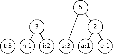
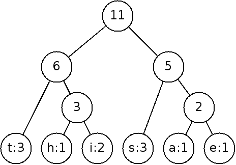
To implement this, we need to keep track of the nodes that we can link and choose the smallest weight each time. This is best done with a priority queue (heap)!

Create a priority queue of nodes such that they are ordered by smallest probability.
Create a leaf node for each input symbol, and add it to the queue.
While there is more than one node in the queue:
1. Remove the two next nodes from the queue.
2. Create a node linking these two as children, with probability of the two children summed.
3. Add this node to the queue.
The one node in the queue is now the root of the complete tree with probability = 1.0

What is the Big-O of this algorithm?