Chapter 1: The Road Ahead

---

 

1.1 What is Computer Science?

---

This book is an introduction to the field of computer science, so we will begin by talking about what computer science is. Unlike other areas, like biology or history, this may not be that obvious. People often are confused about what computer science actually is all about. In particular, it is not any of the following things:

• The study of how to build computer hardware (this is “computer engineering”).
• The practice of setting up computer systems and installing things on them (this is “information technology”).
• The use of computer applications such as email clients, word processors and spreadsheets (this is “computer literacy”).

Instead, computer science is all about algorithms. An algorithm is a detailed, step-by-step procedure for solving a particular problem. Algorithms are essentially instructions that tell us how to solve a problem from beginning to end. They are similar to recipes. When you follow a recipe, you also perform the instructions given one by one. The difference is that the result of your work when following a recipe is a food of some kind (hopefully cake). The result of your work following an algorithm is a solution to a problem.

The study of algorithms actually predates the existence of computers by thousands of years ¹. One of the first known algorithms was described by the Greek mathematician Euclid in his book Elements around 300 BCE. The algorithm was to find the greatest common divisor between two numbers. For example, the greatest common divisor of 12 and 30 is 6 because 6 is the biggest number that goes into both 12 and 30 evenly. We’ll take a look at Euclid’s algorithm in Chapter 6.

Other mathematicians devised algorithms for solving other problems, such as adding, multiplying, factorizing, finding roots of equations, etc. The word “algorithm” itself comes from the name of Muḥammad ibn Mūsā al-Khwārizmī, a Persian mathematician who wrote on algorithms for solving algebra and arithmetic problems. The word “algebra” also comes from the title of one of al-Khwārizmī’s books.

You actually have learned several of these sorts of mathematical algorithms yourself while in school. For example, if I asked you to add 137 to 226, you could do so (even though you probably have never added these specific numbers before). That’s because you learned an algorithm as a child for adding numbers like this. That algorithm will allow you to add any two numbers by following its step-by-step process.

One really important aspect of algorithms is that you can use them to solve problems whether or not you understand how the algorithm is working. This was important in the past because it meant you only had to be really clever once, to come up with the algorithm in the first place. After that you, and anyone else, could just follow the algorithm’s instructions to solve new problems with it. As a child, you didn’t have to understand all of the logic behind the adding algorithm to use it. Nowadays this is even more important because most algorithms are not followed by people, but by computers. Computers don’t understand anything, but they can be made to follow the steps of an algorithm automatically.

 

1.2 Algorithm Design

---

One major part of computer science is designing algorithms. As we will see throughout this book, there are many problems that can be solved with a good algorithm. Designing algorithms can be a fun and challenging activity. It involves both sides of your brain in that it takes both logic and creativity to do.

Let’s look at an example of an algorithm to solve the “guess the number” game. In the simplest version of this game, one player thinks of a number between 1 and some upper limit. Then the other player guesses which number they picked until they get it.

Let’s say that Mark and Sofia are playing this game with an upper limit of 10. The game might go like this:

    Mark: I'm thinking of a number between 1 and 10.
    Sofia: Is it 7?
    Mark: No.
    Sofia: Is it 3?
    Mark: No.
    Sofia: Is it 2?
    Mark: No.
    Sofia: Is it 8?
    Mark: Yes.

In this case, Sofia solved the problem by eventually guessing Mark’s number. Now we’ll consider writing an algorithm which will always solve the game, no matter what number Mark picks.

Sofia tried numbers in a sort of random order until she hit on the right one. Most people would do this, but it isn’t really necessary. Instead we could just start at 1, and then guess 2, and then 3 and so on until we get the right number. So this particular algorithm won’t solve the problem the same way a person might, but that’s OK. An algorithm for doing this could be written as:

Algorithm 1

1. Set G to 1.
2. Ask if their number is G.
3. If it was, then we are done!
4. If it was not, then add 1 to G.
5. Go back to step 2.

This algorithm ² works by keeping track of which number we are going to be guessing next, which we call “G”. This is a variable, which is a very important concept in programming. A variable is a name that we give to a value which may change as the algorithm is run. They are like variables in math, but are used somewhat differently. In math, you often have to solve for a variable which has one value that you just need to find. In computer science, variables change values as the algorithm progresses. Here, G starts off at 1, but it will change.

In step 2, we ask the other player if their number is G or not. Of course we don’t ask them if they literally picked “G”. Only numbers are allowed in this game, not letters! Instead the algorithm means that we should instead ask if their number is the current value of G, whatever that happens to be. The first time it will be 1, but as we have said, G will change.

In step 3 and 4, we are going to do different things based on whether or not the guess was correct. If it was, then the algorithm is done. If not, we add 1 to the variable G. When the algorithm first reaches this step, it will change G from 1 to 2.

Step 5 is crucial here. It tells us to go back to step 2. This creates a loop, which is when an algorithm does the same step or steps multiple times. Even though only step 2 makes a guess, the algorithm can keep on guessing numbers because of the loop.

We’ll now trace through the algorithm to see how it works. Let’s suppose that we pick 3 as our number and see if the algorithm can guess it. The algorithm will go step by step as follows:

1. It will start with step 1 and set G to 1.
2. Next it will go onto step 2 and ask us if the number is G (currently 1).
3. We will respond that no, it is not.
4. The algorithm will then skip over step 3 (we aren’t done yet) and go to step 4.
5. In step 4, the algorithm will add 1 to G. Now G is going to be 2.
6. Step 5 will then move the algorithm back to step 2.
7. Back at step 2, the algorithm will ask us if the number is G (which is now equal to 2).
8. We will tell it no.
9. The algorithm will again skip over step 3 and go to step 4.
10. In step 4, the algorithm will again add 1 to G. This changes it from 2 to 3.
11. Step 5 sends the algorithm back to step 2 again.
12. The algorithm will again ask us if the number is G (which is now 3).
13. This time, we tell it yes, since our number was 3.
14. The algorithm then sees this in step 3 and stops.

One important part of working with algorithms is testing them. This involves stepping through the algorithm line by line like this to see how it’s working. Hopefully you’re convinced that the algorithm will try every number until it gets the right one.

 

1.3 Another Version of the Game

---

Next we will look at a more interesting variation of this game. In this variation, instead of just answering “no” for an incorrect guess, the player will either say that the guess was too low, or too high. Again, consider an example with two players. This time, the limit will be 100:

Mark: I'm thinking of a number between 1 and 100.
Sofia: Is it 50?
Mark: Too high.
Sofia: Is it 25?
Mark: Too low.
Sofia: Is it 37?
Mark: Too low.
Sofia: Is it 44?
Mark: Too high.
Sofia: Is it 40?
Mark: Yes.

This time, Sofia did not just guess numbers randomly until she hit on the right one. By having the extra information, she’s able to guess more intelligently. Her first guess of 50 was the best she could have done to start with. The reason is because that way, no matter what Mark answered, she had half the potential numbers eliminated. When Mark said 50 was too high, Sofia knew the number must have been between 1 and 49. Had Mark instead answered that 50 was too low, then Sofia would know the number had to be between 51 and 100. Either way, half the possibilities were cut out.

Sofia used this trick again with her second guess. When she knew the number was between 1 and 49, she guessed right in the middle, which gave her 25. To get this “middle value”, we can just add the numbers and divide by 2. She kept on doing this until she hit on the right number. This algorithm can be given like this:

Algorithm 2

1. Set min to 1.
2. Set max to 100.
3. Set G to (max + min) ÷ 2 (rounding down if needed).
4. Ask if their number is G.
5. If it is, then we are done!
6. If the guess was too high, set max to (G - 1).
7. If the guess was too low, set min to (G + 1).
8. Go back to step 3.

This algorithm is just bit more complicated than the last one. Now we have three variables involved. min is used to keep track of the smallest number the other player could be thinking of. Likewise max keeps track of the biggest number it could be. For example, if we have narrowed it down so we know the number is between 20 and 40, then min would be 20 and max would be 40. These variables will change as we narrow down the possibilities. G is once again used for the number we are going to guess.

The algorithm starts by setting min and max to reflect the fact that the number could be anywhere between 1 and 100 to start with. Then step 3 figures out which number to guess. The first time we do this, we will get 100 plus 1, divided by 2, which gives 50.5. The note about rounding down if needed is to make sure we always guess a whole number, in this case 50.

After each guess, there are 3 possibilities. If we got the guess right, then we are done, just like before. If we guessed too high, then that means that we need to change our max variable. We set it to whatever our last guess was, minus 1. To see why, consider the starting case where min is 1, max is 100, and G is 50. If the guess of 50 was too high, then the number must be between 1 and 49. So we 49 as the new max value. Similar logic holds for when the guess was too low.

Finally we go back to step 3 to pick a new guess again. This algorithm will eventually guess the correct number for playing this version of the game. I would encourage you to try it yourself once or twice to convince yourself that it works.

The things these two algorithms are doing, such as changing variables, checking different conditions, and going back to previous steps, are the same things pretty much all the algorithms we will look at in this book will do. You’ll see that we can use these building blocks to solve all kinds of interesting problems.

 

1.4 Algorithm Analysis

---

Another major part of computer science is analyzing algorithms. Oftentimes a problem will have more than one algorithm to solve it. We then will want to compare the algorithms and see which takes less steps. We now have two algorithms we can analyze. Notice that we could use both algorithms for the second variant of the game (where the player answers too low or too high instead of just no). The first algorithm would just guess starting at 1 all the way up until it got the number. But which algorithm is better? And by how much? These are the questions of algorithm analysis.

When analyzing algorithms, we want to know how many steps they take in different cases. We often consider the average case or the worst case. The average case is helpful because it gives you an idea of how long the algorithm will usually take. The worst case is helpful because it gives you a guarantee on how long it will take. If the algorithm performs well enough in the worst case, you know it will work well for you. The best case is usually not very interesting. Here we will focus on the worst case.

Let’s consider algorithm 1 first (the one that just starts at 1, then 2, then 3, etc.). If we are playing the game between 1 and 100, what’s the most number of guesses that the algorithm could take? Clearly the worst case is that the other player chose 100 as his or her number, because that would be the algorithm’s last guess. In this case, we would have to make 100 guesses before we get it right. If we were playing between 1 and 1,000 then we would need 1,000 guesses in the worst case.

Analyzing algorithm 2 is more complicated. The worst case with this algorithm is that we never “get lucky” by guessing the number correctly until we are 100% sure of what it is. We are only 100% sure when we have narrowed down the range to 1 number, and min and max are the same value. Below is an example of when this could happen:

> min = 1, max = 100.  Is your number 50?
Too high.
> min = 1, max = 49.  Is your number 25?
Too low.
> min = 26, max = 49.  Is your number 37?
Too low.
> min = 38, max = 49.  Is your number 43?
Too high.
> min = 38, max = 42.  Is your number 40?
Too high.
> min = 38, max = 39.  Is your number 38?
Too low.
> min = 39, max = 39.  Is your number 39?
Yes.

As you can see, the algorithm was not lucky enough to get the number right until the very end when it had eliminated all the other possibilities. In this worst case it took 7 guesses to get the number. There are other worst case numbers, but they all take 7 guesses to reach.

The number 7 here comes from the number of times we can cut the possibilities in half before we run out. There were 100 possibilities to begin with, and with each guess we eliminate half of them. If we repeatedly divide 100 by 2 (rounding down because we eliminate the guessed number itself as well), then we get this sequence of numbers:

100
50
25
12
6
3
1

Because we can cut 100 in half 7 times before we hit 1, our algorithm takes 7 guesses in the worst case ³. Below is a table showing the number of guesses needed in the worst case for both algorithms, based on the highest number the other player could pick:

Highest Number	Algorithm 1 Guesses	Algorithm 2 Guesses
10	10	4
100	100	7
1,000	1,000	10
1,000,000	1,000,000	20
1,000,000,000	1,000,000,000	30

It is sort of amazing that we can ask algorithm 2 to guess a number between 1 and 1 billion, and it will need only 30 guesses at most to get it! Algorithm 2 is not just a bit better for this problem, it’s way better. If you were to follow Algorithm 2 with a billion as the highest number, you’d be done in a few minutes. If you used Algorithm 1, and you guess one number per second (with no breaks for eating and sleeping), it would take you more than 31 years.

It’s actually pretty common in computer science for there to be huge differences in speed between different approaches like this. Oftentimes the obvious solution is not very efficient, but a more clever one is. This book will spend more time on algorithm design than analysis, but it is an important part of computer science and we will touch on it from time to time.

 

1.5 Another Algorithm Example

---

Let’s look at another example of an algorithm. Imagine you were asked to add up all of the numbers from 1 to 100. When coming up with an algorithm for a problem I find it’s best to begin thinking about how you would solve the problem manually. In this case, we might follow steps like the following:

1. Start by writing down our first number, 1.
2. Take the second number and add it to the first giving us 3. Here we’ll scratch out the 1 and replace it with the 3.
3. Move to the next number, which is 3 and add it in, giving us 6. Again we replace the 3 with the 6.
4. Move to the 4, and again add it in…

Thinking this through, there’s basically two things we are keeping track of: which number we are currently on, and what our total sum is so far. In algorithms, the way we keep track of things is with variables. So let’s make a variable called current for keeping track of what number we’re on, and one called sum for keeping track of the running total.

With these variables, the algorithm might look like this:

Algorithm 3

1. Set current to 1.
2. Set sum to 0.
3. Set the sum equal to the current sum + current.
4. If current is equal to 100, stop we are done.
5. Add one to current, moving to the next number.
6. Go back to step 3.

This algorithm will run through all the numbers 1 to 100 and compute the total. If we were to give it to a careful and patient person, they would find that the sum is equal to 5,050. We could also write this algorithm in a language that a computer can understand (a topic we’ll spend most of the rest of this book covering) and the computer would be able to give us that answer much more quickly and with no chance of a mistake.

However, this problem also happens to have a more efficient algorithm! The more efficient algorithm was supposedly discovered by the mathematician Carl Friedrich Gauss when he was in elementary school. The story (which may or may not be apocryphal) goes that Gauss’s teacher gave him exactly this problem to keep him occupied and was surprised when Gauss came back after only a few minutes. The way Gauss solved the problem was by realizing you could rewrite the numbers like this:

  1 +   2 +   3 +   4 + ... +  98 +  99 + 100
100 +  99 +  98 +  97 + ... +   3 +   2 +   1
---------------------------------------------
101 + 101 + 101 + 101 + ... + 101 + 101 + 101

The first row is the numbers 1 through 100 added together. The second is the numbers 100 through 1 added together (which results in the same sum of course). When we add the two sets of numbers together like this, every column is equal to 101. To add the one hundred 101’s together we don’t actually need to add. We can just multiply 101 times 100, giving us 10,100. Then we need to divide by 2, because we added two sets of numbers 1 to 100 instead of one. That gives us the answer 5,050 just as the other algorithm did.

Using this technique, we can write a faster algorithm. For clarity, we’ll make a variable for the number we are adding up to, which could be 100 or any other number we wish. We’ll call this variable “N”.

Algorithm 4

1. Set the ending number, N, to 100.
2. Set sum = ((N + 1) * N) / 2

Despite being perhaps harder to understand, algorithm 4 is more efficient than algorithm 3 for solving this problem. To add the numbers 1 through 100, we would do 99 additions with algorithm 3. With algorithm 4, we would do one addition, one multiplication, and one division. Like the guess the number example, the differences between these algorithms also increases as we look at bigger numbers:

Highest Number	Algorithm 3 Operations	Algorithm 4 Operations
10	9	3
100	99	3
1,000	999	3
1,000,000	999,999	3
1,000,000,000	999,999,999	3

Again the choice of algorithm can be very important in terms of how long it takes to solve a problem!

 

1.6 What is a Computer?

---

Computer science is primarily the study of algorithms, but computers do play a role as well. In this section we will talk about what computers are, what programs are, and how computers can run programs.

It might seem a bit silly to define what a computer is, since you likely use a computer every day and clearly know what one is. However, we will define a computer as any device that is capable of running algorithms automatically. The earliest computers were created to run a handful of particular algorithms, and couldn’t do anything else.

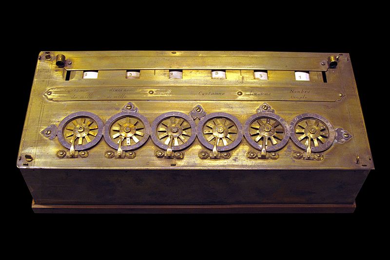
One of the earliest such devices was Pascal’s calculator, also called a Pascaline. This device, created by the French mathematician Blaise Pascal in the mid-1600s, was capable of adding and subtracting numbers. It could also do multiplication and division by means of repeated additions or subtractions. A number of other mathematicians and inventors made similar mechanical devices, including Gottfried Wilhelm Leibniz.

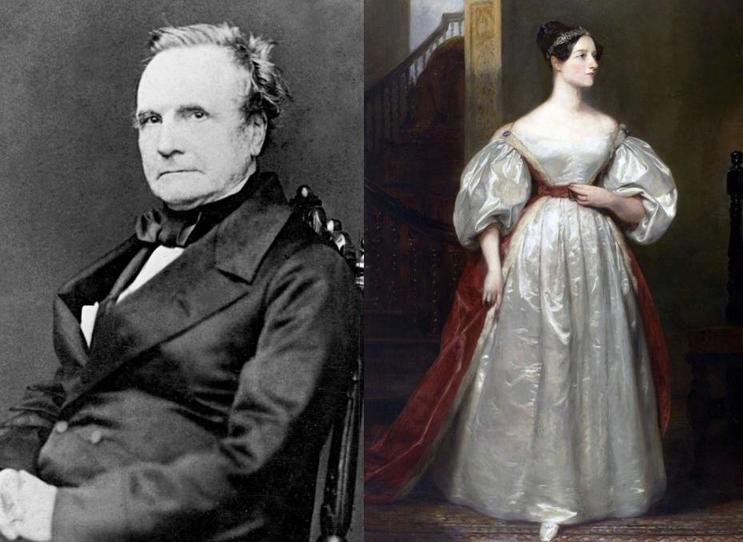
Another pioneer in early computers was the British mathematician and engineer Charles Babbage. He designed the difference engine, which could compute polynomial values. He completed a prototype of the difference engine in 1822. The difference engine was mechanical and was operated with a hand crank. He began working on a larger version which could operate on bigger numbers, with more precision.

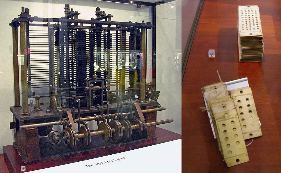
Before the full difference engine was completed, however, Babbage began working on a more ambitious project, the analytical engine. Babbage’s design of the analytical engine was a huge breakthrough in computer science, because it was the first design for a programmable computer. Pascal’s calculator, the difference engine, and every other computing device up until that point was designed to do one fixed task. If you wanted it to solve a different problem, you had to build an entirely new machine.

The analytical engine, on the other hand, was designed so that it could execute any algorithm at all. It did this by taking the instructions that it should execute as input, along with data values to be used in the computation. These sets of instructions are the world’s first computer programs. The analytical engine’s programs themselves were created by punching holes in cards. The machine would then read the cards in, and the patterns of holes would affect its behavior.

Babbage worked with Ada Lovelace, who was incidentally the daughter of the poet Lord Byron. She worked on translating algorithms so that they could be executed by the analytical engine. The first of these was a program to compute the Bernoulli numbers. This was the first published computer program. A program is an algorithm or collection of algorithms that is written specifically for a computer to execute. Unlike Babbage and others at the time, Lovelace believed the analytical engine to be capable of going beyond number crunching, including speculating that the engine could be used to create music.

Unfortunately, the analytical engine was never completed, primarily due to a lack of funding. A general-purpose computer was not actually completed until more than 100 years after the design of the analytical engine. In the 1940s, there were several working computers developed. These include the Z4 by the German Konrad Zuse, the Colossus developed in Great Britain to break coded messages, and the ENIAC developed at the University of Pennsylvania to calculate ballistics trajectories.

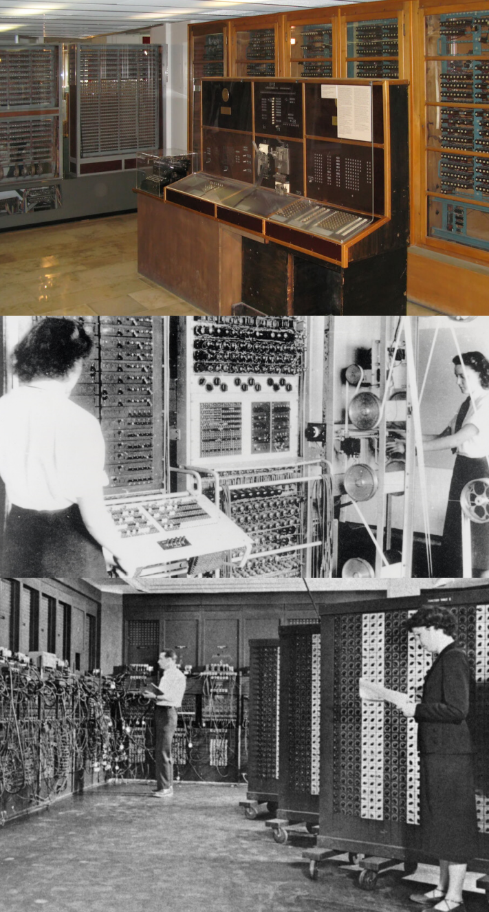
Unlike the Analytical Engine, which was completely mechanical, these computers used electronic circuitry. After these machines were successfully built and used, there was no turning back, and computers have been constantly built and improved upon until the present day.

Despite being as large as rooms, these older computer were laughably limited compared to even the most basic of today’s computers. The Z4 ran at 40 Hz and had 512 bytes of memory. The first iPhone, released in 2007, could run at 620 MHz (15 million times faster), and came with at least 4 GB of memory (7 million times more).

While these older computers were woefully slow and had tiny memories, they functioned in essentially the same way as every computer designed since. They all consist of a processor, memory and some input/output devices. Below is a simplified diagram of a computer system.

The CPU (which stands for central processing unit), is responsible for carrying out the instructions of a program. Each instruction is very simple and precise. For example, the following are examples of typical CPU instructions:

• Take the numbers in two memory cells add them together. Put the answer in another memory cell.
• Check if one memory cell is equal to another. If so, jump to a different part of the program.
• Check if a certain key on the keyboard is pressed. If so, set a memory cell to 1. Otherwise, set it to 0.

Although the individual instructions a CPU carries out are very basic, enough of them put together are able to accomplish great things.

The memory of a computer is responsible for storing numbers. Everything represented in a computer is done with numbers. For instance, when you send an email, the text that you write must be stored inside the computer as well. But, like everything else, this is done with numbers. The letters and punctuation symbols have specific numbers assigned to them. For instance when you type an ‘A’, the computer stores a 65. When you type a period, the computer stores a 46. When you type a space, the computer stores a 32 ⁴.

Of course, the way that computers store numbers is in binary, which means they only use 1’s and 0’s. We will not talk about how to convert back and forth between binary and decimal numbers. Just know that any number can be stored in either binary or decimal, and they mean the same thing. Even images and sounds are stored inside a computer as numbers. We will talk about how that is done in later chapters.

Input devices include touch screens, mice, keyboards, game controllers and so on. These are connected to a computer system so that the user can influence the programs running on the computer. Likewise, output devices are connected to a computer so that the user can see what the computer is doing and see the result of the program which is running. These include monitors, speakers, printers, and vibration units (which can vibrate to provide the user feedback).

 

1.7 Programming Languages

---

So the computer executes simple instructions, reads and writes its memory, gets input from the user, and gives the user output. But where do the instructions come from? They are actually stored inside the computer’s memory as numbers too! As an example of a computer instruction, we can look at one of the steps of Algorithm 1 to solve the simple guess the number game:

add 1 to g.

Let’s look at what this step would look like as a real computer instruction ⁵. But first, we would need to decide what memory location to store G in. Let’s say we put it in location 7.

This instruction would tell the CPU to add 1 to memory location 7:

          operation     destination   input   amount
1110001   0100       0  0111          0111    00000001 0000

This is a binary number. We’ll just point out some of the parts of this. The 0100 labeled “operation” tells the CPU what sort of thing it’s doing. 0100 is the code for addition. So it tells the CPU to add instead of subtract, multiply, or anything else.

The first 0111 labeled “destination” tells the CPU where to put the result. 0111 is binary for 7. So it puts the answer in memory cell 7. The second 0111, labeled “input” tells the CPU what value to read in the addition. This is also 7. Lastly the 00000001 labeled “amount” tells the CPU how much to add. In total the instruction tells the CPU to read memory cell 7, add 1 to it, and put the answer back in memory cell 7.

The other, unlabelled parts just tell the CPU what type of instruction it is, and how to interpret the other fields. All together the instruction is the following binary number:

11100010100001110111000000010000

In decimal, this is equal to:

3800526864

So the way computers work is by reading in these numbers, which tell them what they are supposed to do. Part of the computer’s memory is dedicated to storing these instruction numbers for the programs it runs. It reads the instructions one by one and carries them out. Programs stored as actual numbers like this are machine code programs.

In case you are panicking right now, let me assure you that nobody actually writes programs this way! Giving a computer a program by writing a sequence of numbers like this would be tedious beyond belief.

Instead, we have created other languages which are easier for people to use. The first of these is assembly language, which is basically a human-readable version of machine code. Rather than write “0100” for add, and “0111” for memory cell 7, we just write them out. The instruction above written in assembly would look like this:

add r7, r7, #1

The computer can’t run this instruction directly, it must be translated into machine code. That is done by a program called an assembler:

The assembler converts each line of assembly code into the corresponding machine code instruction. Then, the machine code program can be run on the computer system directly.

We aren’t dealing with numbers directly with assembly code, but it is still too tedious for most people. In particular, we still have to keep track of where in memory our variables are stored. Knowing that memory cell 7 is storing our guess variable, and knowing where the other variables are becomes too hard as we begin to write larger programs.

Instead, we have developed high-level programming languages. These allow us to have names for our variables, instead of needing to remember which memory location they are in. Here is what the instruction above looks like in Python, the high-level language used in this book:

guess = guess + 1

High-level language code is also much more succinct than assembly or machine code. One line of code in a language like Python can do the same work as many lines of machine code. Of course this code must also be translated into machine code for the computer to execute. That is done with a program called an interpreter.

An interpreter takes code in a language like Python, and executes in line by line. For each line it sees, it gives one or more lines of machine code to the computer:

Just like someone who interprets one spoken language into another, an interpreter program translates on the fly. As the high-level program is being run, its code is being translated for the computer to execute.

 

1.8 What do you do with Computer Science?

---

We have seen that computer science is primarily about algorithms, but this section will address how algorithms are used in a variety of areas to solve problems in the world.

Computer science is an interesting field because it frequently works together with other fields. For example:

• Computer scientists work with natural scientists in fields like physics, chemistry and biology to develop computer models of natural phenomenon. It is often impractical to carry out experiments in real life, so computer models can be used. For instance, there are programs which model the collision of two galaxies, the spread of a disease through a population, or the path of a river in the face of flooding. These models allow scientists to test hypotheses and compare potential solutions to problems more easily than they otherwise could.
• Social scientists work with computer scientists as well. For example, economists work with programmers to create programs which model the way markets work. Computer scientists also work with historians and anthropologists to create virtual exhibits for historical artifacts.
• Computer programs are also used in every area of industry. Programs determine the price of goods, they schedule flights, they manage factories and farms, and keep track of information in schools and hospitals. They are behind all of the web sites and apps that you use, and provide entertainment in the form of video games and special effects used in movies.

Some computer scientists work in “pure” computer science. These include people who work on operating systems or the interpreters that make languages like Python work. But the vast majority work with people in some other area. Because so many different fields rely on programs, a computer scientist can work in a variety of different areas over the course of their career. All of this makes computer science an interesting and rewarding field of study. No matter what you’re interested in, computer science can combine with it in some way.

Computer science also has a lower “barrier of entry” than most other fields. You don’t need any special equipment or materials. You can use just about any sort of computer to write your programs (some people assume you need a powerful or specific type of machine, but that’s not the case). It is also a field where you should feel free to experiment. Unlike a chemistry student mixing up chemicals, there’s really not much you can do while programming that will cause any harm to you or your computer.

 

1.9 Comprehension Questions

---

1. What is an algorithm, and what role do algorithms play in computer science?
2. In the context of algorithms, what is a variable?
3. In the context of algorithms, what is a loop?
4. Why is it important that algorithms can be followed without understanding how they work?
5. Why is it important to analyse how long algorithms take?
6. What was special about the Analytical Engine developed by Babbage and Lovelace?
7. Why do most programmers use high-level languages instead of machine language?
8. Give an example of how another field or industry makes use of computer science.

 

1.10 Algorithm Exercises

---

1. Write an algorithm that can find the largest number in a list of 10 numbers. Begin by thinking about what information you will need to keep track of.

2. Below is Euclid’s algorithm for finding the greatest common divisor between two numbers:

   1. Set M to the biggest of our two numbers
   2. Set N to the other number
   3. If N is equal to 0, the answer is M.
   4. Set R to the remainder of M divided by N.
   5. Set M to N.
   6. Set N to R.
   7. Go to step 3.

   What does this algorithm give as the answer with the following inputs:

   1. 30 and 12

   2. 20 and 10

   3. 5 and 3

   Remember that you don’t need to understand why this algorithm works to follow its steps (or indeed even know what a greatest common divisor even is).

3. In grade school you learned an algorithm for adding numbers with any number of digits. Try writing out the algorithm as a set of detailed step-by-step instructions. You can assume that the person following the algorithm can add any 1-digit numbers together (i.e. they can do 7+8 in their head, but can’t add the whole number that way).

Footnotes

---

1. Before the advent of computers, the study of algorithms was not called “computer science”. It was just part of mathematics. After computers were invented, it split off into its own field.↩︎

2. This algorithm is written in “pseudocode” which is not real computer code, but is similar to computer code. For most of this book we will use real code, but for these first examples, we just want to talk about the concepts in general.↩︎

3. For the mathematically inclined, the worst case number of guesses has the following relationship with the number of possibilities we start with: guesses = ⌈log₂(possibilities)⌉↩︎

4. These numbers are defined by the ASCII (American Standard Code for Information Interchange) code. Computer scientists do not need to remember these!↩︎

5. The instruction in this example is for ARM-based computer systems. These include almost all phones, tablets and other small computers. Most laptops and desktops use a different format, but the ideas are the same.↩︎

Copyright © 2019–2023 Ian Finlayson
Licensed under a Creative Commons Attribution 4.0 International License.