Algorithm Analysis

Measuring Algorithm Speed

There are usually many algorithms that solve the same problem. Oftentimes some of these algorithms are more efficient than others.

As we've discussed, the choice between different data structures also has a big effect on the efficiency of programs. For example, removing something from a linked list is a lot faster than removing something from an array. Likewise, adding to the end of a doubly-linked list is a lot faster than adding to the end of a singly-linked list.

But how much faster are these things? Today we'll look at ways of measuring how efficient different algorithms and data structures are.

Using Execution Time

One way of measuring how fast an algorithm is is to actually time it. We can write multiple programs, compile them, and run them to see which one runs faster.

This program adds a number of integers to the end of a singly-linked list.

This program adds a number of integers to the end of a doubly-linked list.

If we try running these programs, we'll see the affect of using a singly vs. doubly linked list. If we only add a few elements, the program is so fast that it makes little difference. Storing a lot of data, however, and the difference becomes clear:

Number of Elements	Singly-Linked	Doubly-Linked
100	.07 s	.08 s
1,000	.09 s	.07 s
10,000	.22 s	.09 s
50,000	3.40 s	.11 s
100,000	13.31 s	.12 s
200,000	56.06 s	.14 s
500,000	18 m	0.27 s

As you can see, the difference is enormous, the singly linked list takes longer and longer when the number being added gets bigger, while the doubly linked list grows much more slowly. With the largest input size, the doubly linked list took 4000 times longer.

Timing programs can give a very clear idea of how efficient a given program is. But there are some major drawbacks:

It only can really compare two algorithms. Timing only one program doesn't give you an objective measure of its speed. If we only ran the test on the singly linked list, then we wouldn't necessarily know if it's efficient or not.
There is a large variation in the time it takes to run a program. Notice that when we increased the input size of the doubly-linked list program from 100 to 1000, the time actually went down. That doesn't really make sense, but is caused by the fact that computers run more than one program at a time. Also the second time you run the same program is usually faster than the first time, since the code is loaded into the computer's cache.
It only gives you a measure of a whole program — not individual functions or algorithms. That means to test a single algorithm, we'd need to write a program that contains only that.
You need to test multiple input sizes. If we only tested up to a thousand, there would have been little difference.

Order of Growth

An alternative way to quantify the efficiency of an algorithm is to express it in terms how much more work we have to do for larger and larger inputs. The algorithm to add a node at the end of a singly-linked list is given below:

Create the new node with the right data.
Set the new node's next field to NULL.
If the list is empty, set the head to the new node and return.
Search through the list from the head for the last node:
1. Check if this node is last.
2. If not, move onto the next node.
Set the last node's next field to the new node.

If we have an empty list, this algorithm will not need to loop at all looking for the end, so the algorithm will have 4 steps. If we have 10 items, the algorithm will loop through all 10 items to find the end, and have 24 steps (20 for the loop and 4 for the others). If we have 100 items, the algorithm will loop through all 100 to find the end, and have 204 steps. With 1000 items, the algorithm will have 2004 steps.

We could write a function to give us the number of steps the algorithm takes as a function of the size of the linked list like this:

$steps(n) = 2 \cdot n + 4$

Now we can say how many steps are needed for any input size. However, this is a bit too precise than we actually want to be. In algorithm analysis, we are just looking for a rough idea of how many steps an algorithm takes.

In this case, when we start having more and more nodes, it should be clear that the loop dominates the algorithm. The fact that there are 4 extra steps doesn't really matter.

Likewise, the fact that there are two steps in the loop doesn't really matter. When we turn this algorithm into a program, the loop could have more or less Java instructions (for example you can sometimes do things in one line of code or two, depending on how you write it). Likewise, the compiler can turn a Java instruction into any number of machine instructions.

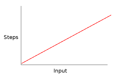
So in algorithm analysis, we will just say this algorithm takes $O(n)$ steps. That comes from removing the coefficient of 2, and the constant of 4. What this tells us is that the number of steps scales linearly with the size of the linked list.

A graph where the x axis is the input size, the y axis is the number
of stpes. The graph depicts a diagonal line. — $O(n)$

Big-O Notation

Big-O notation is how algorithm efficiency is expressed. It basically expresses how the runtime of an algorithm scales with the input. In Big-O notation, the algorithm above is expressed as $O(n)$.

The $O$ stands for "order of" and the $n$ is how big the input to the algorithm is. So with an input size of $n$ (the number of things in the linked list), this algorithm take around $n$ steps to complete.

Big-O lets us capture the most important aspect of an algorithm without getting lost in details like how many seconds it takes to run, or figuring out exactly how many machine code instructions it needs to accomplish some task.

The algorithm for adding to the end of a doubly linked list is given below:

Make the new node with the given data.
Set the node's next to NULL.
If the list is empty:
1. Set the head to node.
2. Set the tail to node.
3. Set node's prev to NULL.
Otherwise:
1. Set node's prev to tail.
2. Set tail's next to node.
3. Set tail to node.

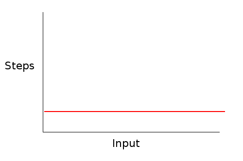
There is no loop in this algorithm. It will always take the same number of steps no matter how big or small the list is. Again, the exact number doesn't matter. Whether it's 6 instructions, 5 instructions, or 25 instructions, the number won't change based on how big the list is. This means that the algorithm is constant time. This is expressed as $O(1)$ in Big-O notation.

A graph where the x axis is the input size, the y axis is the number
of stpes. The graph depicts a horizontal line. — $O(1)$

The smaller the complexity, the better. So $O(1)$ is better than $O(n)$. Note, however, that for small values of $n$, a $O(n)$ algorithm could actually run faster. For example, adding to an empty singly-linked list could be faster than adding to an empty doubly-linked list. However, what happens with larger input sizes is generally all we care about.