Pipelining is a general optimization technique to increase the speed of a some task. The main idea is that you break the task down into multiple stages. For instance, suppose we are doing laundry, which we can break into the following stages:
If we have only one load of laundry to do, it would take 110 minutes. However, if we have multiple loads of laundry to do, we can overlap the different stages. When we move the first load from the washer to the dryer, we put the second load into the washer.
If we had two loads of laundry to do, how long will it take? 3? 100?
Instruction pipelining is exactly the same idea, but applied to the different things we need to do to execute an instruction. Unlike laundry, we can divide the execution of an instruction up in many different ways.
The more stages we make, the less time each one will take, and the faster we can make our clock run. However, the more pipeline stages we have, the more complex the processor is, and the more overhead due to pipelining (such as saving temporary results).
Below are the number of pipeline stages for some common processors:
As we will see, pipelining instruction execution is not quite so simple as it is with laundry. There are a few complications which need to be handled.
The ARM7TDMI processor used in the Game Boy Advance is a very simple three stage pipeline where the stages are:
Fetch
Read the next instruction from memory.
Decode
Decode the instruction into multiple signals, and also read registers.
Execute
Perform an ALU operation, and write a register. Perform a memory operation on load or store.
Suppose we want to execute our version of the strlen function:
@ strlen.s

/* assembly version of strlen */
.global mystrlen
mystrlen:
    mov r1, #0
top:
    ldrb r2, [r0, r1]
    cmp r2, #0
    beq done
    add r1, r1, #1
    b top
done:
    mov r0, r1
    mov pc, lr
Suppose we call this with the argument "Hi". How would this actually run through the 3 stage pipeline?
What kind of speed up would pipelining give us, assuming that each stage takes about one third of the time?
There are a few instances of data hazards in the above program. A data hazard is a case when a value we wish to read has not finished being written yet.
For instance, in these two instructions:
add r0, r0, #1
mul r2, r0, r1
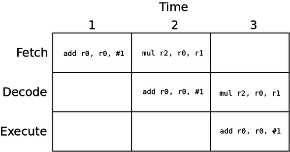
We write code like this a lot, but when we pipeline it, the r0 value is not actually written by the add instruction by the time the mul instruction goes to read it:

The issue is that the value of r0 is not written into the register file until the add instruction has finished executing, at the end of cycle 3. However, the mul instruction tries to read r0 during cycle 3. The value is not ready yet, which is the hazard.
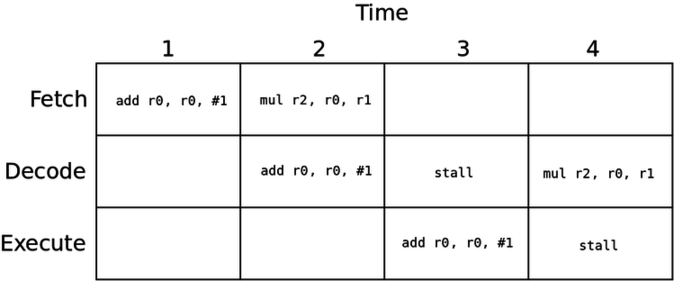
One approach to fix this issue is to simply stall the pipeline. Detect that register 0 is not ready, and make the mul instruction simply wait one cycle.

This slows things down, but avoids reading an incorrect value.
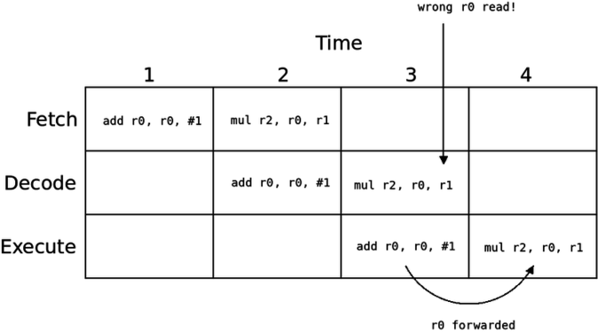
A better approach to fixing data hazards is forwarding wherein we just let the instruction read the incorrect value, but then replace it with the right value before it is used:

Here, we simply let the mul instruction read the stale r0 register. However, by the time mul gets to the execute stage, r0 is ready. We simply use that value which was just computed as the input to the ALU in place of the incorrect value we read.
Data forwarding is widely used with pipelining in order to avoid pipeline stalls.
There is another issue with the program above. Consider these two lines:
    beq done
    add r1, r1, #1
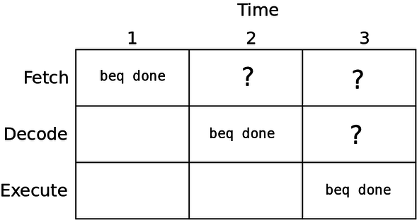
The issue with this is that the branch is resolved during the end of the execute stage. This means that we do not actually know where we are going until the end of the execute stage, which is after when we would fetch the next instruction:

Which instruction should we fetch after the beq? The next instruction, or the one at the done label?
There are two approaches to solving this problem:
The first approach is very simple, but will not be efficient. The second avoids some stalls, and is not very difficult to implement. This is likely the approach taken by the GBA processor.
The GBA processor definitely does not take the last approach which is used by most modern processors with longer pipelines. This approach is called "branch prediction".
Branch prediction is a scheme wherein we simply try to guess whether a branch will be taken or not. There are a variety of branch prediction schemes:
Static Prediction
The simplest form of branch prediction always makes the same prediction for each branch. Typically this means we will predict that backwards branches are taken (because they are probably loops). We can predict that forward branches are taken or not taken based on something else: heuristics or programmer hints.
Global Prediction
In this scheme, we keep a history of our $N$ most recent branches. For instance, if $N$ is 4, then we will have one byte whose bits indicate the 4 branches we most recently executed. A 0 indicates that we did not take a branch, and a 1 indicates that we did.
We use this number to index a table of predictions. For instance, if we have a branch history value of 1001, then we will index a 16-entry table with the value 9. This table will tell us whether to predict this branch as taken or not.
Local Prediction
With local prediction, instead of a global branch history, we keep the branch history of every individual branch. Each time we see a branch, we look up its history using the lower bits to index a history table. For instance, if we store 256 branch's history, then we use the lower 8 bits to look up its history.
We use this value to index the prediction table, which will tell us if the branch should be predicted taken or not.
This usually works better than global prediction because we have information specific to each individual branch, but is more costly in terms of energy and area.
Combined Prediction
Here, we keep both local, and global prediction and combine them in some way. We could predict a branch both ways and then use a "meta-predictor" to choose which of the two schemes to determine which result to use.
High performance processors use large, complex branch predictors which achieve very good results (well over 95% correct).
Another issue with branch prediction is that, even if we know that a branch will be taken ahead of time, we still need to know its target address! For instance, with the beq done instruction, how do we know the address of done? In fact ARM uses PC-relative branches, so we only know that we are branching $N$ instructions past the current PC value.
Normally, this addition is done during the execute stage. In order to know the address ahead of time, branch predictors use another table called the branch target buffer to store the addresses.
As stated the ARM7TDMI processor does not do branch prediction. It can afford not to since the pipeline has just three stages. This means that a stall is not that costly when compared to longer pipelines. The ARM architecture also has a feature which can be used to avoid branches: conditional execution.
With conditional execution we can make an instruction depend on the result of a previous compare instruction. To do this, we append one of the following condition codes to our opcode:
| Condition Code | Only executed when |
| eq | Equal |
| ne | Not equal |
| gt | Greater than |
| lt | Less than |
| ge | Greater than or equal to |
| le | Less than or equal to |
For instance, our original abs function was written as:
.global abs
abs:
    cmp r0, #0
    bge .end
    mvn r1, r0
    add r0, r1, #1
.end:
    mov pc, lr
However we can in fact avoid using a branch at all if we make the mvn and add instructions conditional:
.global abs
abs:
    cmp r0, #0
    mvnlt r1, r0
    addlt r0, r1, #1
    mov pc, lr
The mvnlt and addlt instructions will always execute, i.e. they will always fill pipeline stages. However, they will only have an effect in the case when the cmp instruction produced a "less than" result.
How many cycles will each of these programs take?
Copyright © 2025 Ian Finlayson | Licensed under a Creative Commons BY-NC-SA 4.0 License.